import os
import sys
import pathlib
import numpy as np
## import seaborn as sns
import matplotlib.pyplot as plt
import copy
## from pprint import pprint ##.

path = pathlib.Path(os.getcwd())
module_path = str(path.parent) + '/'
sys.path.append(module_path)

from pymdp.agent import Agent
from pymdp import utils
from pymdp.maths import softmax

import matplotlib.pyplot as plt
from matplotlib.gridspec import GridSpec
from matplotlib.lines import Line2D
from matplotlib.ticker import MaxNLocatorWe use PyMDP and modify an existing demo:
https://github.com/infer-actively/pymdp/blob/master/examples/agent_demo.ipynb
The modifications are:
Do some restructuring of the contents
Use some of my preferred symbols
Use the
_carprefix (for cardinality of factors and modalities)Add a
_labdict for all labelsUse implied label indices from _lab to set values of matrices
Add visualization
Prefix globals with
_Lines where changes were made usually contains
##.structure highest level of content based on interaction pairs
use math symbols with superscripts indicating agent identity
change sta –> s in _lab dict
change obs –> o in _lab dict
change ctr –> u in _lab dict
reorder main loop steps to act, future, next, observe, infer, slide
change idx –> val for value
partition _lab dict to separate agt & sus labels
Active Inference Demo: Constructing a basic generative model from the “ground up”
This demo notebook provides a full walk-through of how to build a POMDP agent’s generative model and perform active inference routine (inversion of the generative model) using the Agent() class of pymdp. We build a generative model from ‘ground up’, directly encoding our own A, B, and C matrices.
First, import pymdp and the modules we’ll need.
## ?utils.get_model_dimensions_from_labels
##.rewrite method to allow for shorter names so that the _lab dict can be used more
##   easily when setting up the matrices
def get_model_dimensions_from_labels(model_labels):
    ## modalities = model_labels['observations']
    modalities = model_labels['o'] ##.
    num_modalities = len(modalities.keys())
    num_obs = [len(modalities[modality]) for modality in modalities.keys()]

    ## factors = model_labels['states']
    factors = model_labels['s'] ##.
    num_factors = len(factors.keys())
    num_states = [len(factors[factor]) for factor in factors.keys()]

    ## if 'actions' in model_labels.keys():
    if 'u' in model_labels.keys(): ##.
        ## controls = model_labels['actions']
        controls = model_labels['u'] ##.
        num_control_fac = len(controls.keys())
        num_controls = [len(controls[cfac]) for cfac in controls.keys()]
        return num_obs, num_modalities, num_states, num_factors, num_controls, num_control_fac
    else:
        return num_obs, num_modalities, num_states, num_factors
1 Player/Game interaction
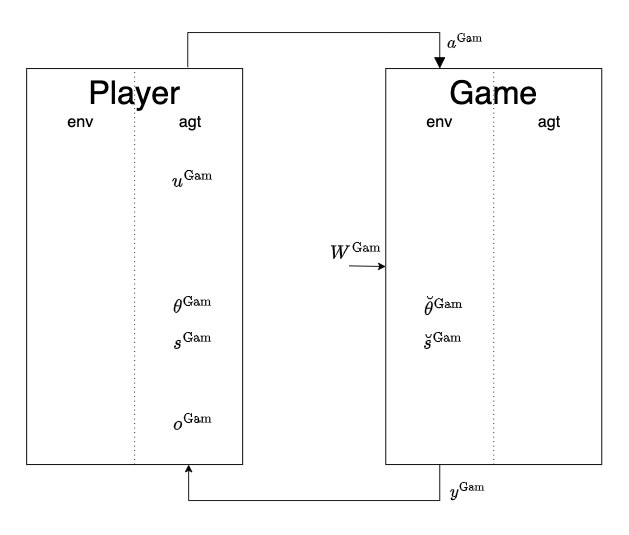
The following diagram is a representation of the interaction between the Player and the Game.
The Game entity (envir) has symbols:
- \(a^{\mathrm{Gam}}\) is the action on the Game entity
- \(\breve\theta^{\mathrm{Gam}}\) is the true parameters of the Game entity
- \(\breve s^{\mathrm{Gam}}\) is the true state of the Game entity
- \(W^{\mathrm{Gam}}\) is the exogenous information impacting the Game entity
- \(y^{\mathrm{Gam}}\) is the observation from the Game entity
The Player entity (agent) has symbols:
- \(u^{\mathrm{Gam}}\) is the inferred action states of the Game entity
- \(\theta^{\mathrm{Gam}}\) is the inferred parameters of the Game entity
- \(s^{\mathrm{Gam}}\) is the inferred state of the Game entity
- \(y^{\mathrm{Gam}}\) is the predicted observation of the Game entity
1.1 Player agent
This is the agent’s generative model for the game environment which embodies the system-under-steer for the player/game interaction.
1.1.1 State factors
We assume the agent’s “represents” (this should make you think: generative model , not process ) its environment using two latent variables that are statistically independent of one another - we can thus represent them using two hidden state factors.
We refer to these two hidden state factors as
- \(s^{\mathrm{Gam}}_1\) (GAME_STATE)
- \(s^{\mathrm{Gam}}_2\) (PLAYING_VS_SAMPLING)
1.1.1.1 \(s^{\mathrm{Gam}}_1\) (GAME_STATE)
The first factor is a binary variable representing some ‘reward structure’ that characterises the world. It has two possible values or levels:
- one level that will lead to rewards with high probability
- \(s^{\mathrm{Gam}}_1 = 0\), a state/level we will call
HIGH_REW, and
- \(s^{\mathrm{Gam}}_1 = 0\), a state/level we will call
- another level that will lead to “punishments” (e.g. losing money) with high probability
- \(s^{\mathrm{Gam}}_1 = 1\), a state/level we will call
LOW_REW
- \(s^{\mathrm{Gam}}_1 = 1\), a state/level we will call
You can think of this hidden state factor as describing the ‘pay-off’ structure of e.g. a two-armed bandit or slot-machine with two different settings - one where you’re more likely to win (HIGH_REW), and one where you’re more likely to lose (LOW_REW). Crucially, the agent doesn’t know what the GAME_STATE actually is. They will have to infer it by actively furnishing themselves with observations
1.1.1.2 \(s^{\mathrm{Gam}}_2\) (PLAYING_VS_SAMPLING)
The second factor is a ternary (3-valued) variable representing the decision-state or ‘sampling state’ of the agent itself.
- The first state/level of this hidden state factor is just the
- starting or initial state of the agent
- \(s^{\mathrm{Gam}}_2 = 0\), a state that we can call
START
- \(s^{\mathrm{Gam}}_2 = 0\), a state that we can call
- starting or initial state of the agent
- the second state/level is the
- state the agent occupies when “playing” the multi-armed bandit or slot machine
- \(s^{\mathrm{Gam}}_2 = 1\), a state that we can call
PLAYING
- \(s^{\mathrm{Gam}}_2 = 1\), a state that we can call
- state the agent occupies when “playing” the multi-armed bandit or slot machine
- the third state/level of this factor is a
- “sampling state”
- \(s^{\mathrm{Gam}}_2 = 2\), a state that we can call
SAMPLING - This is a decision-state that the agent occupies when it is “sampling” data in order to find out the level of the first hidden state factor - the GAME_STATE \(s^{\mathrm{Gam}}_1\).
- \(s^{\mathrm{Gam}}_2 = 2\), a state that we can call
- “sampling state”
1.1.2 Observation modalities
The observation modalities themselves are divided into 3 modalities. You can think of these as 3 independent sources of information that the agent has access to. You could think of this in direct perceptual terms - e.g. 3 different sensory organs like eyes, ears, & nose, that give you qualitatively-different kinds of information. Or you can think of it more abstractly - like getting your news from 3 different media sources (online news articles, Twitter feed, and Instagram).
1.1.2.1 \(o^{\mathrm{Gam}}_1\) (Observations of the game state, GAME_STATE_OBS)
The first observation modality is the \(o^{\mathrm{Gam}}_1\) (GAME_STATE_OBS) modality, and corresponds to observations that give the agent information about the GAME_STATE \(s^{\mathrm{Gam}}_1\). There are three possible outcomes within this modality:
HIGH_REW_EVIDENCE- \(o^{\mathrm{Gam}}_1 = 0\)
LOW_REW_EVIDENCE- \(o^{\mathrm{Gam}}_1 = 1\)
NO_EVIDENCE- \(o^{\mathrm{Gam}}_1 = 2\)
So the first outcome can be described as lending evidence to the idea that the GAME_STATE \(s^{\mathrm{Gam}}_1\) is HIGH_REW; the second outcome can be described as lending evidence to the idea that the GAME_STATE \(s^{\mathrm{Gam}}_1\) is LOW_REW; and the third outcome within this modality doesn’t tell the agent one way or another whether the GAME_STATE \(s^{\mathrm{Gam}}_1\) is HIGH_REW or LOW_REW.
1.1.2.2 \(o^{\mathrm{Gam}}_2\) (Reward observations, GAME_OUTCOME)
The second observation modality is the \(o^{\mathrm{Gam}}_2\) (GAME_OUTCOME) modality, and corresponds to arbitrary observations that are functions of the GAME_STATE \(s^{\mathrm{Gam}}_1\). We call the first outcome level of this modality
REWARD- \(o^{\mathrm{Gam}}_2 = 0\), which gives you a hint about how we’ll set up the C matrix (the agent’s “utility function” over outcomes). We call the second outcome level of this modality
PUN- \(o^{\mathrm{Gam}}_2\) = 1, and the third outcome level
NEUTRAL- \(o^{\mathrm{Gam}}_2 = 2\)
By design, we will set up the A matrix such that the REWARD outcome is (expected to be) more likely when the GAME_STATE \(s^{\mathrm{Gam}}_1\) is HIGH_REW (0) and when the agent is in the PLAYING state, and that the PUN outcome is (expected to be) more likely when the GAME_STATE \(s^{\mathrm{Gam}}_1\) is LOW_REW (1) and the agent is in the PLAYING state. The NEUTRAL outcome is not expected to occur when the agent is playing the game, but will be expected to occur when the agent is in the SAMPLING state. This NEUTRAL outcome within the \(o^{\mathrm{Gam}}_2\) (GAME_OUTCOME) modality is thus a meaningless or ‘null’ observation that the agent gets when it’s not actually playing the game (because an observation has to be sampled nonetheless from all modalities).
1.1.2.3 \(o^{\mathrm{Gam}}_3\) (“Proprioceptive” or self-state observations, ACTION_SELF_OBS)
The third observation modality is the \(o^{\mathrm{Gam}}_3\) (ACTION_SELF_OBS) modality, and corresponds to the agent observing what level of the \(s^{\mathrm{Gam}}_2\) (PLAYING_VS_SAMPLING) state it is currently in. These observations are direct, ‘unambiguous’ mappings to the true \(\breve{s}^{\mathrm{Gam}}_2\) (PLAYING_VS_SAMPLING) state, and simply allow the agent to “know” whether it’s playing the game, sampling information to learn about the game state, or where it’s sitting at the START state. The levels of this outcome are simply thus
START_O,PLAY_O, andSAMPLE_O,
where the _O suffix simply distinguishes them from their corresponding hidden states, for which they provide direct evidence.
Note about the arbitrariness of ‘labelling’ observations, before defining the A and C matrices.
There is a bit of a circularity here, in that that we’re “pre-empting” what the A matrix (likelihood mapping) should look like, by giving these observations labels that imply particular roles or meanings. An observation per se doesn’t mean anything, it’s just some discrete index that distinguishes it from another observation. It’s only through its probabilistic relationship to hidden states (encoded in the A matrix, as we’ll see below) that we endow an observation with meaning. For example: by already labelling \(o^{\mathrm{Gam}}_1 = 0\) (GAME_STATE_OBS) as HIGH_REW_EVIDENCE, that’s a hint about how we’re going to structure the A matrix for the \(o^{\mathrm{Gam}}_1\) (GAME_STATE_OBS) modality.
_labPlrGam = { ## labels for Player/Game (agent/environment) interaction
    ## agt
    "u": {
        "uᴳᵃᵐ₁": [ ## "NULL"
            "NULL_ACTION",
        ],
        "uᴳᵃᵐ₂": [ ## "PLAYING_VS_SAMPLING_CONTROL"
            "START_ACTION",
            "PLAY_ACTION",
            "SAMPLE_ACTION"
        ],
    },
    "s": {
        "sᴳᵃᵐ₁": [ ## "GAME_STATE"
            "HIGH_REW",
            "LOW_REW"
        ],
        "sᴳᵃᵐ₂": [ ## "PLAYING_VS_SAMPLING"
            "START",
            "PLAYING",
            "SAMPLING"
        ],
    },
    "o": {
        "oᴳᵃᵐ₁": [ ## "GAME_STATE_OBS"
            "HIGH_REW_EVIDENCE",
            "LOW_REW_EVIDENCE",
            "NO_EVIDENCE"
        ],
        "oᴳᵃᵐ₂": [ ## "GAME_OUTCOME"
            "REWARD",
            "PUN",
            "NEUTRAL"
        ],
        "oᴳᵃᵐ₃": [ ## "ACTION_SELF_OBS", direct obser of hidden state PLAYING_VS_SAMPLING
            "START_O",
            "PLAY_O",
            "SAMPLE_O"
        ]
    },
    ## env/sus
    "a": {
        "aᴳᵃᵐ₁": [ ## "NULL"
            "NULL_ACTION",
        ],
        "aᴳᵃᵐ₂": [ ## "PLAYING_VS_SAMPLING_CONTROL"
            "START_ACTION",
            "PLAY_ACTION",
            "SAMPLE_ACTION"
        ],
    },
    "s̆": {
        "s̆ᴳᵃᵐ₁": [ ## "GAME_STATE"
            "HIGH_REW",
            "LOW_REW"
        ],
        "s̆ᴳᵃᵐ₂": [ ## "PLAYING_VS_SAMPLING"
            "START",
            "PLAYING",
            "SAMPLING"
        ],
    },
    "y": {
        "yᴳᵃᵐ₁": [ ## "GAME_STATE_OBS"
            "HIGH_REW_EVIDENCE",
            "LOW_REW_EVIDENCE",
            "NO_EVIDENCE"
        ],
        "yᴳᵃᵐ₂": [ ## "GAME_OUTCOME"
            "REWARD",
            "PUN",
            "NEUTRAL"
        ],
        "yᴳᵃᵐ₃": [ ## "ACTION_SELF_OBS", direct obser of hidden state PLAYING_VS_SAMPLING
            "START_O",
            "PLAY_O",
            "SAMPLE_O"
        ]
    },
}
_car_o,_num_o, _car_s,_num_s, _car_u,_num_u = get_model_dimensions_from_labels(_labPlrGam) ##.
_car_o,_num_o, _car_s,_num_s, _car_u,_num_u
([3, 3, 3], 3, [2, 3], 2, [1, 3], 2)print(f'{_car_u=}') ##.cardinality of control factors
print(f'{_num_u=}') ##.number of control factors
print(f'{_car_s=}') ##.cardinality of state factors
print(f'{_num_s=}') ##.number of state factors
print(f'{_car_o=}') ##.cardinality of observation modalities
print(f'{_num_o=}') ##.number of observation modalities_car_u=[1, 3]
_num_u=2
_car_s=[2, 3]
_num_s=2
_car_o=[3, 3, 3]
_num_o=3##.
_u_fac_names = list(_labPlrGam['u'].keys()); print(f'{_u_fac_names=}') ##.control factor names
_s_fac_names = list(_labPlrGam['s'].keys()); print(f'{_s_fac_names=}') ##.state factor names
_o_mod_names = list(_labPlrGam['o'].keys()); print(f'{_o_mod_names=}') ##.observation modality names_u_fac_names=['uᴳᵃᵐ₁', 'uᴳᵃᵐ₂']
_s_fac_names=['sᴳᵃᵐ₁', 'sᴳᵃᵐ₂']
_o_mod_names=['oᴳᵃᵐ₁', 'oᴳᵃᵐ₂', 'oᴳᵃᵐ₃']##.
_a_fac_names = list(_labPlrGam['a'].keys()); print(f'{_a_fac_names=}') ##.control factor names
_s̆_fac_names = list(_labPlrGam['s̆'].keys()); print(f'{_s̆_fac_names=}') ##.state factor names
_y_mod_names = list(_labPlrGam['y'].keys()); print(f'{_y_mod_names=}') ##.observation modality names_a_fac_names=['aᴳᵃᵐ₁', 'aᴳᵃᵐ₂']
_s̆_fac_names=['s̆ᴳᵃᵐ₁', 's̆ᴳᵃᵐ₂']
_y_mod_names=['yᴳᵃᵐ₁', 'yᴳᵃᵐ₂', 'yᴳᵃᵐ₃']Setting up observation likelihood matrix - first main component of generative model
## A = utils.obj_array_zeros([[o] + _car_state for _, o in enumerate(_car_obser)]) ##.
_Aᴳᵃᵐ = utils.obj_array_zeros([[car_o] + _car_s for car_o in _car_o]) ##.
_Aᴳᵃᵐ
array([array([[[0., 0., 0.],
[0., 0., 0.]],
[[0., 0., 0.],
[0., 0., 0.]],
[[0., 0., 0.],
[0., 0., 0.]]]), array([[[0., 0., 0.],
[0., 0., 0.]],
[[0., 0., 0.],
[0., 0., 0.]],
[[0., 0., 0.],
[0., 0., 0.]]]),
array([[[0., 0., 0.],
[0., 0., 0.]],
[[0., 0., 0.],
[0., 0., 0.]],
[[0., 0., 0.],
[0., 0., 0.]]])], dtype=object)Set up the first modality’s likelihood mapping, correspond to how \(o^{\mathrm{Gam}}_1\) (GAME_STATE_OBS) are related to hidden states.
## they always get the 'no evidence' observation in the START STATE
_Aᴳᵃᵐ[0][ ##.
    _labPlrGam['o']['oᴳᵃᵐ₁'].index('NO_EVIDENCE'),
    :,
    _labPlrGam['s']['sᴳᵃᵐ₂'].index('START')
] = 1.0
## they always get the 'no evidence' observation in the PLAYING STATE
_Aᴳᵃᵐ[0][ ##.
    _labPlrGam['o']['oᴳᵃᵐ₁'].index('NO_EVIDENCE'),
    :,
    _labPlrGam['s']['sᴳᵃᵐ₂'].index('PLAYING')
] = 1.0
## the agent expects to see the HIGH_REW_EVIDENCE observation with 80% probability,
##   if the GAME_STATE is HIGH_REW, and the agent is in the SAMPLING state
_Aᴳᵃᵐ[0][ ##.
    _labPlrGam['o']['oᴳᵃᵐ₁'].index('HIGH_REW_EVIDENCE'),
    _labPlrGam['s']['sᴳᵃᵐ₁'].index('HIGH_REW'),
    _labPlrGam['s']['sᴳᵃᵐ₂'].index('SAMPLING')
] = 0.8
## the agent expects to see the LOW_REW_EVIDENCE observation with 20% probability,
##   if the GAME_STATE is HIGH_REW, and the agent is in the SAMPLING state
_Aᴳᵃᵐ[0][ ##.
    _labPlrGam['o']['oᴳᵃᵐ₁'].index('LOW_REW_EVIDENCE'),
    _labPlrGam['s']['sᴳᵃᵐ₁'].index('HIGH_REW'),
    _labPlrGam['s']['sᴳᵃᵐ₂'].index('SAMPLING')
] = 0.2

## the agent expects to see the LOW_REW_EVIDENCE observation with 80% probability,
##   if the GAME_STATE is LOW_REW, and the agent is in the SAMPLING state
_Aᴳᵃᵐ[0][ ##.
    _labPlrGam['o']['oᴳᵃᵐ₁'].index('LOW_REW_EVIDENCE'),
    _labPlrGam['s']['sᴳᵃᵐ₁'].index('LOW_REW'),
    _labPlrGam['s']['sᴳᵃᵐ₂'].index('SAMPLING')
] = 0.8
## the agent expects to see the HIGH_REW_EVIDENCE observation with 20% probability,
##   if the GAME_STATE is LOW_REW, and the agent is in the SAMPLING state
_Aᴳᵃᵐ[0][ ##.
    _labPlrGam['o']['oᴳᵃᵐ₁'].index('HIGH_REW_EVIDENCE'),
    _labPlrGam['s']['sᴳᵃᵐ₁'].index('LOW_REW'),
    _labPlrGam['s']['sᴳᵃᵐ₂'].index('SAMPLING')
] = 0.2

## quick way to do this
## Aᴳᵃᵐ[0][:, :, 0] = 1.0
## Aᴳᵃᵐ[0][:, :, 1] = 1.0
## Aᴳᵃᵐ[0][:, :, 2] = np.array([[0.8, 0.2], [0.2, 0.8], [0.0, 0.0]])

_Aᴳᵃᵐ[0]
array([[[0. , 0. , 0.8],
[0. , 0. , 0.2]],
[[0. , 0. , 0.2],
[0. , 0. , 0.8]],
[[1. , 1. , 0. ],
[1. , 1. , 0. ]]])Set up the second modality’s likelihood mapping, correspond to how \(o^{\mathrm{Gam}}_2\) (GAME_OUTCOME) are related to hidden states.
## regardless of the game state, if you're at the START, you see the 'neutral' outcome
_Aᴳᵃᵐ[1][ ##.
    _labPlrGam['o']['oᴳᵃᵐ₂'].index('NEUTRAL'),
    :,
    _labPlrGam['s']['sᴳᵃᵐ₂'].index('START')
] = 1.0

## regardless of the game state, if you're in the SAMPLING state, you see the 'neutral' outcome
_Aᴳᵃᵐ[1][ ##.
    _labPlrGam['o']['oᴳᵃᵐ₂'].index('NEUTRAL'),
    :,
    _labPlrGam['s']['sᴳᵃᵐ₂'].index('SAMPLING')
] = 1.0

## this is the distribution that maps from the "GAME_STATE" to the "GAME_OUTCOME"
##   observation , in the case that "GAME_STATE" is `HIGH_REW`
_HIGH_REW_MAPPING = softmax(np.array([1.0, 0]))

## this is the distribution that maps from the "GAME_STATE" to the "GAME_OUTCOME"
##   observation , in the case that "GAME_STATE" is `LOW_REW`
_LOW_REW_MAPPING = softmax(np.array([0.0, 1.0]))

## fill out the A matrix using the reward probabilities
_Aᴳᵃᵐ[1][ ##.
    _labPlrGam['o']['oᴳᵃᵐ₂'].index('REWARD'),
    _labPlrGam['s']['sᴳᵃᵐ₁'].index('HIGH_REW'),
    _labPlrGam['s']['sᴳᵃᵐ₂'].index('PLAYING')
] = _HIGH_REW_MAPPING[0]
_Aᴳᵃᵐ[1][ ##.
    _labPlrGam['o']['oᴳᵃᵐ₂'].index('PUN'),
    _labPlrGam['s']['sᴳᵃᵐ₁'].index('HIGH_REW'),
    _labPlrGam['s']['sᴳᵃᵐ₂'].index('PLAYING')
] = _HIGH_REW_MAPPING[1]
_Aᴳᵃᵐ[1][ ##.
    _labPlrGam['o']['oᴳᵃᵐ₂'].index('REWARD'),
    _labPlrGam['s']['sᴳᵃᵐ₁'].index('LOW_REW'),
    _labPlrGam['s']['sᴳᵃᵐ₂'].index('PLAYING')
] = _LOW_REW_MAPPING[0]
_Aᴳᵃᵐ[1][ ##.
    _labPlrGam['o']['oᴳᵃᵐ₂'].index('PUN'),
    _labPlrGam['s']['sᴳᵃᵐ₁'].index('LOW_REW'),
    _labPlrGam['s']['sᴳᵃᵐ₂'].index('PLAYING')
] = _LOW_REW_MAPPING[1]

## quick way to do this
## Aᴳᵃᵐ[1][2, :, 0] = np.ones(num_states[0])
## Aᴳᵃᵐ[1][0:2, :, 1] = softmax(np.eye(num_obs[1] - 1)) # relationship of game state to reward observations (mapping between reward-state (first hidden state factor) and rewards (Good vs Bad))
## Aᴳᵃᵐ[1][2, :, 2] = np.ones(num_states[0])

_Aᴳᵃᵐ[1]
array([[[0. , 0.73105858, 0. ],
[0. , 0.26894142, 0. ]],
[[0. , 0.26894142, 0. ],
[0. , 0.73105858, 0. ]],
[[1. , 0. , 1. ],
[1. , 0. , 1. ]]])Set up the third modality’s likelihood mapping, correspond to how \(o^{\mathrm{Gam}}_3\) (ACTION_SELF_OBS) are related to hidden states.
_Aᴳᵃᵐ[2][ ##.
_labPlrGam['o']['oᴳᵃᵐ₃'].index('START_O'),
:,
_labPlrGam['s']['sᴳᵃᵐ₂'].index('START')
] = 1.0
_Aᴳᵃᵐ[2][ ##.
_labPlrGam['o']['oᴳᵃᵐ₃'].index('PLAY_O'),
:,
_labPlrGam['s']['sᴳᵃᵐ₂'].index('PLAYING')
] = 1.0
_Aᴳᵃᵐ[2][ ##.
_labPlrGam['o']['oᴳᵃᵐ₃'].index('SAMPLE_O'),
:,
_labPlrGam['s']['sᴳᵃᵐ₂'].index('SAMPLING')
] = 1.0
## quick way to do this
## modality_idx, factor_idx = 2, 2
## for sampling_state_i in num_states[factor_idx]:
## Aᴳᵃᵐ[modality_idx][sampling_state_i,:,sampling_state_i] = 1.0
_Aᴳᵃᵐ[2]array([[[1., 0., 0.],
[1., 0., 0.]],
[[0., 1., 0.],
[0., 1., 0.]],
[[0., 0., 1.],
[0., 0., 1.]]])print(f'=== _car_s:\n{_car_s}')
print(f'=== _car_o:\n{_car_o}')
_Aᴳᵃᵐ=== _car_s:
[2, 3]
=== _car_o:
[3, 3, 3]array([array([[[0. , 0. , 0.8],
[0. , 0. , 0.2]],
[[0. , 0. , 0.2],
[0. , 0. , 0.8]],
[[1. , 1. , 0. ],
[1. , 1. , 0. ]]]),
array([[[0.        , 0.73105858, 0.        ],
        [0.        , 0.26894142, 0.        ]],

       [[0.        , 0.26894142, 0.        ],
        [0.        , 0.73105858, 0.        ]],

       [[1.        , 0.        , 1.        ],
[1. , 0. , 1. ]]]),
array([[[1., 0., 0.],
        [1., 0., 0.]],

       [[0., 1., 0.],
        [0., 1., 0.]],

       [[0., 0., 1.],
[0., 0., 1.]]])], dtype=object)1.1.3 Control factors
The ‘control state’ factors are the agent’s representation of the control states (or actions) that it believes can influence the dynamics of the hidden states - i.e. hidden state factors that are under the influence of control states are are ‘controllable’. In practice, we often encode every hidden state factor as being under the influence of control states, but the ‘uncontrollable’ hidden state factors are driven by a trivially-1-dimensional control state or action-affordance. This trivial action simply ‘maintains the default environmental dynamics as they are’ i.e. does nothing. This will become more clear when we set up the transition model (the B matrices) below.
1.1.3.1 \(u^{\mathrm{Gam}}_1\) (NULL)
This reflects the agent’s lack of ability to influence the GAME_STATE \(s^{\mathrm{Gam}}_1\) using policies or actions. The dimensionality of this control factor is 1, and there is only one action along this control factor:
NULL_ACTIONor “don’t do anything to do the environment”.
This just means that the transition dynamics along the GAME_STATE \(s^{\mathrm{Gam}}_1\) hidden state factor have their own, uncontrollable dynamics that are not conditioned on this \(u^{\mathrm{Gam}}_1\) (NULL) control state - or rather, always conditioned on an unchanging, 1-dimensional NULL_ACTION.
1.1.3.2 \(u^{\mathrm{Gam}}_2\) (PLAYING_VS_SAMPLING_CONTROL)
This is a control factor that reflects the agent’s ability to move itself between the START, PLAYING and SAMPLING states of the \(s^{\mathrm{Gam}}_2\) (PLAYING_VS_SAMPLING) hidden state factor. The levels/values of this control factor are
START_ACTIONPLAY_ACTIONSAMPLE_ACTION
When we describe the B matrices below, we will set up the transition dynamics of the \(s^{\mathrm{Gam}}_2\) (PLAYING_VS_SAMPLING) hidden state factor, such that they are totally determined by the value of the \(u^{\mathrm{Gam}}_2\) (PLAYING_VS_SAMPLING_CONTROL) factor.
(Controllable-) Transition Dynamics
Importantly, some hidden state factors are controllable by the agent, meaning that the probability of being in state \(i\) at \(t+1\) isn’t merely a function of the state at \(t\), but also of actions (or from the generative model’s perspective, control states ). So each transition likelihood or B matrix encodes conditional probability distributions over states at \(t+1\), where the conditioning variables are both the states at \(t-1\) and the actions at \(t-1\). This extra conditioning on control states is encoded by a third, lagging dimension on each factor-specific B matrix. So they are technically B “tensors” or an array of action-conditioned B matrices.
For example, in our case the 2nd hidden state factor \(s^{\mathrm{Gam}}_2\) (PLAYING_VS_SAMPLING) is under the control of the agent, which means the corresponding transition likelihoods B[1] are index-able by both previous state and action.
## this is the (non-trivial) controllable factor, where there will be a >1-dimensional
##   control state along this factor
_control_fac_idx = [1] ##.used in Agent constructor
_Bᴳᵃᵐ = utils.obj_array(_num_s) ##.
_Bᴳᵃᵐ
array([None, None], dtype=object)_Bᴳᵃᵐ[0] = np.zeros((_car_s[0], _car_s[0], _car_u[0])) ##.
_Bᴳᵃᵐ[0]array([[[0.],
[0.]],
[[0.],
[0.]]])_p_stoch = 0.0
## we cannot influence factor zero, set up the 'default' stationary dynamics -
## one state just maps to itself at the next timestep with very high probability,
## by default. So this means the reward state can change from one to another with
## some low probability (p_stoch)
_Bᴳᵃᵐ[0][ ##.
_labPlrGam['s']['sᴳᵃᵐ₁'].index('HIGH_REW'),
_labPlrGam['s']['sᴳᵃᵐ₁'].index('HIGH_REW'),
_labPlrGam['u']['uᴳᵃᵐ₁'].index('NULL_ACTION')
] = 1.0 - _p_stoch
_Bᴳᵃᵐ[0][ ##.
_labPlrGam['s']['sᴳᵃᵐ₁'].index('LOW_REW'),
_labPlrGam['s']['sᴳᵃᵐ₁'].index('HIGH_REW'),
_labPlrGam['u']['uᴳᵃᵐ₁'].index('NULL_ACTION')
] = _p_stoch
_Bᴳᵃᵐ[0][ ##.
_labPlrGam['s']['sᴳᵃᵐ₁'].index('LOW_REW'),
_labPlrGam['s']['sᴳᵃᵐ₁'].index('LOW_REW'),
_labPlrGam['u']['uᴳᵃᵐ₁'].index('NULL_ACTION')
] = 1.0 - _p_stoch
_Bᴳᵃᵐ[0][ ##.
_labPlrGam['s']['sᴳᵃᵐ₁'].index('HIGH_REW'),
_labPlrGam['s']['sᴳᵃᵐ₁'].index('LOW_REW'),
_labPlrGam['u']['uᴳᵃᵐ₁'].index('NULL_ACTION')
] = _p_stoch
_Bᴳᵃᵐ[0]array([[[1.],
[0.]],
[[0.],
[1.]]])## setup our controllable factor
_Bᴳᵃᵐ[1] = np.zeros((_car_s[1], _car_s[1], _car_u[1])) ##.
_Bᴳᵃᵐ[1][ ##.
_labPlrGam['s']['sᴳᵃᵐ₂'].index('START'),
:,
_labPlrGam['u']['uᴳᵃᵐ₂'].index('START_ACTION')
] = 1.0
_Bᴳᵃᵐ[1][ ##.
_labPlrGam['s']['sᴳᵃᵐ₂'].index('PLAYING'),
:,
_labPlrGam['u']['uᴳᵃᵐ₂'].index('PLAY_ACTION')
] = 1.0
_Bᴳᵃᵐ[1][ ##.
_labPlrGam['s']['sᴳᵃᵐ₂'].index('SAMPLING'),
:,
_labPlrGam['u']['uᴳᵃᵐ₂'].index('SAMPLE_ACTION')
] = 1.0
_Bᴳᵃᵐ[1]array([[[1., 0., 0.],
[1., 0., 0.],
[1., 0., 0.]],
[[0., 1., 0.],
[0., 1., 0.],
[0., 1., 0.]],
[[0., 0., 1.],
[0., 0., 1.],
[0., 0., 1.]]])print(f'=== _car_contr:\n{_car_u}')
print(f'=== _car_state:\n{_car_s}')
_Bᴳᵃᵐ=== _car_contr:
[1, 3]
=== _car_state:
[2, 3]array([array([[[1.],
[0.]],
[[0.],
[1.]]]), array([[[1., 0., 0.],
[1., 0., 0.],
[1., 0., 0.]],
[[0., 1., 0.],
[0., 1., 0.],
[0., 1., 0.]],
[[0., 0., 1.],
[0., 0., 1.],
[0., 0., 1.]]])], dtype=object)Prior preferences
Now we parameterise the C vector, or the prior beliefs about observations. This will be used in the expression of the prior over actions, which is technically a softmax function of the negative expected free energy of each action. It is the equivalent of the exponentiated reward function in reinforcement learning treatments.
_Cᴳᵃᵐ = utils.obj_array_zeros([car_o for car_o in _car_o]) ##.
_Cᴳᵃᵐ
array([array([0., 0., 0.]), array([0., 0., 0.]), array([0., 0., 0.])],
dtype=object)## make the observation we've a priori named `REWARD` actually desirable, by building
## a high prior expectation of encountering it
_Cᴳᵃᵐ[1][ ##.
_labPlrGam['o']['oᴳᵃᵐ₂'].index('REWARD'),
] = 1.0
## make the observation we've a prior named `PUN` actually aversive, by building a
## low prior expectation of encountering it
_Cᴳᵃᵐ[1][ ##.
_labPlrGam['o']['oᴳᵃᵐ₂'].index('PUN'),
] = -1.0
## the above code implies the following for the `neutral' observation:
## we don't need to write this - but it's basically just saying that observing `NEUTRAL`
## is in between reward and punishment
_Cᴳᵃᵐ[1][ ##.
_labPlrGam['o']['oᴳᵃᵐ₂'].index('NEUTRAL'),
] = 0.0
_Cᴳᵃᵐ[1]array([ 1., -1., 0.])Initialise an instance of the Agent() class:
All you have to do is call Agent(generative_model_params...) where generative_model_params are your A, B, C’s… and whatever parameters of the generative model you want to specify
_agtPlr = Agent(A=_Aᴳᵃᵐ, B=_Bᴳᵃᵐ, C=_Cᴳᵃᵐ, control_fac_idx=_control_fac_idx)
_agtPlr
<pymdp.agent.Agent at 0x7fbecd4d9660>1.2 Game environment
This is the agent’s generative process for the game environment which embodies the system-under-steer for the player/game interaction.
Important note how the generative process doesn’t have to be described by A and B matrices - can just be the arbitrary ‘rules of the game’ that you ‘write in’ as a modeller. But here we just use the same transition/likelihood matrices to make the sampling process straightforward.
## transition/observation matrices characterising the generative process
## _A_gp = copy.deepcopy(_A)
_Ăᴳᵃᵐ = copy.deepcopy(_Aᴳᵃᵐ) ##.

## _B_gp = copy.deepcopy(_B)
_B̆ᴳᵃᵐ = copy.deepcopy(_Bᴳᵃᵐ) ##.
Initialise the simulation
## initial state
_T = 20 ## number of timesteps in the simulation

_s̆ᴳᵃᵐ = [ ## initial (true) state
    _labPlrGam['s']['sᴳᵃᵐ₁'].index('HIGH_REW'),
    _labPlrGam['s']['sᴳᵃᵐ₂'].index('START')
]; print(f'{_s̆ᴳᵃᵐ=}')

_yᴳᵃᵐ = [ ## initial observation
    _labPlrGam['o']['oᴳᵃᵐ₁'].index('NO_EVIDENCE'),
    _labPlrGam['o']['oᴳᵃᵐ₂'].index('NEUTRAL'),
    _labPlrGam['o']['oᴳᵃᵐ₃'].index('START_O')
]; print(f'{_yᴳᵃᵐ=}')
_s̆ᴳᵃᵐ=[0, 0]
_yᴳᵃᵐ=[2, 2, 0]Create some string names for the state, observation, and action indices to help with print statements
##.value names
_u_val_names = [_labPlrGam['u'][cfn] for cfn in _u_fac_names]; print(f'{_u_val_names=}') ##.
_s_val_names = [_labPlrGam['s'][sfn] for sfn in _s_fac_names]; print(f'{_s_val_names=}') ##.
_o_val_names = [_labPlrGam['o'][omn] for omn in _o_mod_names]; print(f'{_o_val_names=}')

_a_val_names = [_labPlrGam['a'][cfn] for cfn in _a_fac_names]; print(f'{_a_val_names=}') ##.
_s̆_val_names = [_labPlrGam['s̆'][sfn] for sfn in _s̆_fac_names]; print(f'{_s̆_val_names=}') ##.
_y_val_names = [_labPlrGam['y'][omn] for omn in _y_mod_names]; print(f'{_y_val_names=}')
_u_val_names=[['NULL_ACTION'], ['START_ACTION', 'PLAY_ACTION', 'SAMPLE_ACTION']]
_s_val_names=[['HIGH_REW', 'LOW_REW'], ['START', 'PLAYING', 'SAMPLING']]
_o_val_names=[['HIGH_REW_EVIDENCE', 'LOW_REW_EVIDENCE', 'NO_EVIDENCE'], ['REWARD', 'PUN', 'NEUTRAL'], ['START_O', 'PLAY_O', 'SAMPLE_O']]
_a_val_names=[['NULL_ACTION'], ['START_ACTION', 'PLAY_ACTION', 'SAMPLE_ACTION']]
_s̆_val_names=[['HIGH_REW', 'LOW_REW'], ['START', 'PLAYING', 'SAMPLING']]
_y_val_names=[['HIGH_REW_EVIDENCE', 'LOW_REW_EVIDENCE', 'NO_EVIDENCE'], ['REWARD', 'PUN', 'NEUTRAL'], ['START_O', 'PLAY_O', 'SAMPLE_O']]Run simulation
_a_facs = {'aᴳᵃᵐ₁': [], 'aᴳᵃᵐ₂': []}
_s_facs = {'sᴳᵃᵐ₁': [], 'sᴳᵃᵐ₂': []}

_s̆_facs = {'s̆ᴳᵃᵐ₁': [], 's̆ᴳᵃᵐ₂': []}
_y_mods = {'yᴳᵃᵐ₁': [], 'yᴳᵃᵐ₂': [], 'yᴳᵃᵐ₃': []}

## min_F = []
_qIpiIs = []
_GNegs = []
action = np.array([0.0, 0.0]) ##.
for t in range(_T):
    print(f"\nTime {t}:")

    ### act
    print('___ act ___')
    if(t == 0): ##.at t=0 agent has no q_pi yet, so no .sample_action()
        print(f"_aᴳᵃᵐ: {[(_a_fac_names[a], _a_val_names[a][int(action[a])]) for a in range(len(_s̆_fac_names))]}")
    else: ## t > 0
        action = _agtPlr.sample_action()
        ## min_F.append(np.min(_agent.F)) ##.does not have .F
        print(f"_aᴳᵃᵐ: {[(_a_fac_names[a], _a_val_names[a][int(action[a])]) for a in range(len(_s̆_fac_names))]}") ##.
        for afi, afn in enumerate(_a_fac_names):
            _a_facs[afn].append(_a_val_names[afi][int(action[afi])])

    ### future
    print('___ future ___')
    ## _agent.infer_policies()
    qIpiI, GNeg = _agtPlr.infer_policies() ##.posterior over policies and negative EFE
    print(f'{qIpiI=}')
    print(f'{GNeg=}')
    _qIpiIs.append(qIpiI)
    _GNegs.append(GNeg)

    ### next
    print('___ next ___')
    for sfi, sf in enumerate(_s̆ᴳᵃᵐ):
        _s̆ᴳᵃᵐ[sfi] = utils.sample(_B̆ᴳᵃᵐ[sfi][:, sf, int(action[sfi])]) ##.
    print(f"_s̆ᴳᵃᵐ: {[(_s̆_fac_names[sfi], _s̆_val_names[sfi][_s̆ᴳᵃᵐ[sfi]]) for sfi in range(len(_s̆_fac_names))]}") ##.
    for sfi, sfn in enumerate(_s̆_fac_names):
        _s̆_facs[sfn].append(_s̆_val_names[sfi][_s̆ᴳᵃᵐ[sfi]])

    ### observe
    print('___ observe ___')
    for omi, _ in enumerate(_yᴳᵃᵐ): ##.
        _yᴳᵃᵐ[omi] = utils.sample(_Ăᴳᵃᵐ[omi][:, _s̆ᴳᵃᵐ[0], _s̆ᴳᵃᵐ[1]]) ##.
    print(f"_yᴳᵃᵐ: {[(_y_mod_names[omi], _y_val_names[omi][_yᴳᵃᵐ[omi]]) for omi in range(len(_y_mod_names))]}") ##.
    for ymi, ymn in enumerate(_y_mod_names):
        _y_mods[ymn].append(_y_val_names[ymi][_yᴳᵃᵐ[ymi]])

    ### infer
    print('___ infer ___')
    belief_state = _agtPlr.infer_states(_yᴳᵃᵐ) ##.
    print(f"Beliefs: {[(_s_fac_names[sfi], belief_state[sfi].round(3).T) for sfi in range(len(_s_fac_names))]}") ##.
    for sfi, sfn in enumerate(_s_fac_names):
        _s_facs[sfn].append( _labPlrGam['s'][sfn][int(np.argmax(belief_state[sfi].round(3).T))] ) ##.
    ## exmpl: print(f"_s̆ᴳᵃᵐ: {[(_s̆_fac_names[sfi], _s̆_idx_names[sfi][_s̆ᴳᵃᵐ[sfi]]) for sfi in range(len(_s̆_fac_names))]}") ##.
    ## print(f"_sᴳᵃᵐ: {[(_sta_fac_names[sfi], _sta_idx_names[sfi]) for sfi in range(len(_sta_fac_names))]}") ##.
Time 0:
___ act ___
_aᴳᵃᵐ: [('aᴳᵃᵐ₁', 'NULL_ACTION'), ('aᴳᵃᵐ₂', 'START_ACTION')]
___ future ___
qIpiI=array([0.03478899, 0.20528675, 0.75992426])
GNeg=array([-3.60483043, -3.49388625, -3.41208556])
___ next ___
_s̆ᴳᵃᵐ: [('s̆ᴳᵃᵐ₁', 'HIGH_REW'), ('s̆ᴳᵃᵐ₂', 'START')]
___ observe ___
_yᴳᵃᵐ: [('yᴳᵃᵐ₁', 'NO_EVIDENCE'), ('yᴳᵃᵐ₂', 'NEUTRAL'), ('yᴳᵃᵐ₃', 'START_O')]
___ infer ___
Beliefs: [('sᴳᵃᵐ₁', array([0.5, 0.5])), ('sᴳᵃᵐ₂', array([1., 0., 0.]))]
Time 1:
___ act ___
_aᴳᵃᵐ: [('aᴳᵃᵐ₁', 'NULL_ACTION'), ('aᴳᵃᵐ₂', 'SAMPLE_ACTION')]
___ future ___
qIpiI=array([0.03478899, 0.20528675, 0.75992426])
GNeg=array([-3.60483043, -3.49388625, -3.41208556])
___ next ___
_s̆ᴳᵃᵐ: [('s̆ᴳᵃᵐ₁', 'HIGH_REW'), ('s̆ᴳᵃᵐ₂', 'SAMPLING')]
___ observe ___
_yᴳᵃᵐ: [('yᴳᵃᵐ₁', 'HIGH_REW_EVIDENCE'), ('yᴳᵃᵐ₂', 'NEUTRAL'), ('yᴳᵃᵐ₃', 'SAMPLE_O')]
___ infer ___
Beliefs: [('sᴳᵃᵐ₁', array([0.8, 0.2])), ('sᴳᵃᵐ₂', array([0., 0., 1.]))]
Time 2:
___ act ___
_aᴳᵃᵐ: [('aᴳᵃᵐ₁', 'NULL_ACTION'), ('aᴳᵃᵐ₂', 'SAMPLE_ACTION')]
___ future ___
qIpiI=array([0.00362533, 0.96895062, 0.02742404])
GNeg=array([-3.60483043, -3.25556369, -3.47836328])
___ next ___
_s̆ᴳᵃᵐ: [('s̆ᴳᵃᵐ₁', 'HIGH_REW'), ('s̆ᴳᵃᵐ₂', 'SAMPLING')]
___ observe ___
_yᴳᵃᵐ: [('yᴳᵃᵐ₁', 'LOW_REW_EVIDENCE'), ('yᴳᵃᵐ₂', 'NEUTRAL'), ('yᴳᵃᵐ₃', 'SAMPLE_O')]
___ infer ___
Beliefs: [('sᴳᵃᵐ₁', array([0.5, 0.5])), ('sᴳᵃᵐ₂', array([0., 0., 1.]))]
Time 3:
___ act ___
_aᴳᵃᵐ: [('aᴳᵃᵐ₁', 'NULL_ACTION'), ('aᴳᵃᵐ₂', 'PLAY_ACTION')]
___ future ___
qIpiI=array([0.03478899, 0.20528675, 0.75992426])
GNeg=array([-3.60483043, -3.49388625, -3.41208556])
___ next ___
_s̆ᴳᵃᵐ: [('s̆ᴳᵃᵐ₁', 'HIGH_REW'), ('s̆ᴳᵃᵐ₂', 'PLAYING')]
___ observe ___
_yᴳᵃᵐ: [('yᴳᵃᵐ₁', 'NO_EVIDENCE'), ('yᴳᵃᵐ₂', 'REWARD'), ('yᴳᵃᵐ₃', 'PLAY_O')]
___ infer ___
Beliefs: [('sᴳᵃᵐ₁', array([0.731, 0.269])), ('sᴳᵃᵐ₂', array([0., 1., 0.]))]
Time 4:
___ act ___
_aᴳᵃᵐ: [('aᴳᵃᵐ₁', 'NULL_ACTION'), ('aᴳᵃᵐ₂', 'SAMPLE_ACTION')]
___ future ___
qIpiI=array([0.00728806, 0.90734217, 0.08536976])
GNeg=array([-3.60483043, -3.30331282, -3.4510333 ])
___ next ___
_s̆ᴳᵃᵐ: [('s̆ᴳᵃᵐ₁', 'HIGH_REW'), ('s̆ᴳᵃᵐ₂', 'SAMPLING')]
___ observe ___
_yᴳᵃᵐ: [('yᴳᵃᵐ₁', 'HIGH_REW_EVIDENCE'), ('yᴳᵃᵐ₂', 'NEUTRAL'), ('yᴳᵃᵐ₃', 'SAMPLE_O')]
___ infer ___
Beliefs: [('sᴳᵃᵐ₁', array([0.916, 0.084])), ('sᴳᵃᵐ₂', array([0., 0., 1.]))]
Time 5:
___ act ___
_aᴳᵃᵐ: [('aᴳᵃᵐ₁', 'NULL_ACTION'), ('aᴳᵃᵐ₂', 'PLAY_ACTION')]
___ future ___
qIpiI=array([0.00121169, 0.9954936 , 0.00329471])
GNeg=array([-3.60483043, -3.18537893, -3.54231138])
___ next ___
_s̆ᴳᵃᵐ: [('s̆ᴳᵃᵐ₁', 'HIGH_REW'), ('s̆ᴳᵃᵐ₂', 'PLAYING')]
___ observe ___
_yᴳᵃᵐ: [('yᴳᵃᵐ₁', 'NO_EVIDENCE'), ('yᴳᵃᵐ₂', 'PUN'), ('yᴳᵃᵐ₃', 'PLAY_O')]
___ infer ___
Beliefs: [('sᴳᵃᵐ₁', array([0.8, 0.2])), ('sᴳᵃᵐ₂', array([0., 1., 0.]))]
Time 6:
___ act ___
_aᴳᵃᵐ: [('aᴳᵃᵐ₁', 'NULL_ACTION'), ('aᴳᵃᵐ₂', 'PLAY_ACTION')]
___ future ___
qIpiI=array([0.00362533, 0.96895062, 0.02742404])
GNeg=array([-3.60483043, -3.25556369, -3.47836328])
___ next ___
_s̆ᴳᵃᵐ: [('s̆ᴳᵃᵐ₁', 'HIGH_REW'), ('s̆ᴳᵃᵐ₂', 'PLAYING')]
___ observe ___
_yᴳᵃᵐ: [('yᴳᵃᵐ₁', 'NO_EVIDENCE'), ('yᴳᵃᵐ₂', 'REWARD'), ('yᴳᵃᵐ₃', 'PLAY_O')]
___ infer ___
Beliefs: [('sᴳᵃᵐ₁', array([0.916, 0.084])), ('sᴳᵃᵐ₂', array([0., 1., 0.]))]
Time 7:
___ act ___
_aᴳᵃᵐ: [('aᴳᵃᵐ₁', 'NULL_ACTION'), ('aᴳᵃᵐ₂', 'PLAY_ACTION')]
___ future ___
qIpiI=array([0.00121169, 0.9954936 , 0.00329471])
GNeg=array([-3.60483043, -3.18537893, -3.54231138])
___ next ___
_s̆ᴳᵃᵐ: [('s̆ᴳᵃᵐ₁', 'HIGH_REW'), ('s̆ᴳᵃᵐ₂', 'PLAYING')]
___ observe ___
_yᴳᵃᵐ: [('yᴳᵃᵐ₁', 'NO_EVIDENCE'), ('yᴳᵃᵐ₂', 'REWARD'), ('yᴳᵃᵐ₃', 'PLAY_O')]
___ infer ___
Beliefs: [('sᴳᵃᵐ₁', array([0.967, 0.033])), ('sᴳᵃᵐ₂', array([0., 1., 0.]))]
Time 8:
___ act ___
_aᴳᵃᵐ: [('aᴳᵃᵐ₁', 'NULL_ACTION'), ('aᴳᵃᵐ₂', 'PLAY_ACTION')]
___ future ___
qIpiI=array([7.89044066e-04, 9.98014004e-01, 1.19695225e-03])
GNeg=array([-3.60483043, -3.15841165, -3.57878595])
___ next ___
_s̆ᴳᵃᵐ: [('s̆ᴳᵃᵐ₁', 'HIGH_REW'), ('s̆ᴳᵃᵐ₂', 'PLAYING')]
___ observe ___
_yᴳᵃᵐ: [('yᴳᵃᵐ₁', 'NO_EVIDENCE'), ('yᴳᵃᵐ₂', 'REWARD'), ('yᴳᵃᵐ₃', 'PLAY_O')]
___ infer ___
Beliefs: [('sᴳᵃᵐ₁', array([0.988, 0.012])), ('sᴳᵃᵐ₂', array([0., 1., 0.]))]
Time 9:
___ act ___
_aᴳᵃᵐ: [('aᴳᵃᵐ₁', 'NULL_ACTION'), ('aᴳᵃᵐ₂', 'PLAY_ACTION')]
___ future ___
qIpiI=array([6.73423691e-04, 9.98535582e-01, 7.90994555e-04])
GNeg=array([-3.60483043, -3.14847603, -3.59477315])
___ next ___
_s̆ᴳᵃᵐ: [('s̆ᴳᵃᵐ₁', 'HIGH_REW'), ('s̆ᴳᵃᵐ₂', 'PLAYING')]
___ observe ___
_yᴳᵃᵐ: [('yᴳᵃᵐ₁', 'NO_EVIDENCE'), ('yᴳᵃᵐ₂', 'REWARD'), ('yᴳᵃᵐ₃', 'PLAY_O')]
___ infer ___
Beliefs: [('sᴳᵃᵐ₁', array([0.995, 0.005])), ('sᴳᵃᵐ₂', array([0., 1., 0.]))]
Time 10:
___ act ___
_aᴳᵃᵐ: [('aᴳᵃᵐ₁', 'NULL_ACTION'), ('aᴳᵃᵐ₂', 'PLAY_ACTION')]
___ future ___
qIpiI=array([6.35368381e-04, 9.98689779e-01, 6.74852661e-04])
GNeg=array([-3.60483043, -3.14483077, -3.60106234])
___ next ___
_s̆ᴳᵃᵐ: [('s̆ᴳᵃᵐ₁', 'HIGH_REW'), ('s̆ᴳᵃᵐ₂', 'PLAYING')]
___ observe ___
_yᴳᵃᵐ: [('yᴳᵃᵐ₁', 'NO_EVIDENCE'), ('yᴳᵃᵐ₂', 'REWARD'), ('yᴳᵃᵐ₃', 'PLAY_O')]
___ infer ___
Beliefs: [('sᴳᵃᵐ₁', array([0.998, 0.002])), ('sᴳᵃᵐ₂', array([0., 1., 0.]))]
Time 11:
___ act ___
_aᴳᵃᵐ: [('aᴳᵃᵐ₁', 'NULL_ACTION'), ('aᴳᵃᵐ₂', 'PLAY_ACTION')]
___ future ___
qIpiI=array([6.21934035e-04, 9.98742087e-01, 6.35978758e-04])
GNeg=array([-3.60483043, -3.14349182, -3.60343473])
___ next ___
_s̆ᴳᵃᵐ: [('s̆ᴳᵃᵐ₁', 'HIGH_REW'), ('s̆ᴳᵃᵐ₂', 'PLAYING')]
___ observe ___
_yᴳᵃᵐ: [('yᴳᵃᵐ₁', 'NO_EVIDENCE'), ('yᴳᵃᵐ₂', 'REWARD'), ('yᴳᵃᵐ₃', 'PLAY_O')]
___ infer ___
Beliefs: [('sᴳᵃᵐ₁', array([0.999, 0.001])), ('sᴳᵃᵐ₂', array([0., 1., 0.]))]
Time 12:
___ act ___
_aᴳᵃᵐ: [('aᴳᵃᵐ₁', 'NULL_ACTION'), ('aᴳᵃᵐ₂', 'PLAY_ACTION')]
___ future ___
qIpiI=array([6.17066394e-04, 9.98760764e-01, 6.22170077e-04])
GNeg=array([-3.60483043, -3.14299956, -3.60431563])
___ next ___
_s̆ᴳᵃᵐ: [('s̆ᴳᵃᵐ₁', 'HIGH_REW'), ('s̆ᴳᵃᵐ₂', 'PLAYING')]
___ observe ___
_yᴳᵃᵐ: [('yᴳᵃᵐ₁', 'NO_EVIDENCE'), ('yᴳᵃᵐ₂', 'REWARD'), ('yᴳᵃᵐ₃', 'PLAY_O')]
___ infer ___
Beliefs: [('sᴳᵃᵐ₁', array([1., 0.])), ('sᴳᵃᵐ₂', array([0., 1., 0.]))]
Time 13:
___ act ___
_aᴳᵃᵐ: [('aᴳᵃᵐ₁', 'NULL_ACTION'), ('aᴳᵃᵐ₂', 'PLAY_ACTION')]
___ future ___
qIpiI=array([6.15285688e-04, 9.98767559e-01, 6.17155362e-04])
GNeg=array([-3.60483043, -3.14281851, -3.6046408 ])
___ next ___
_s̆ᴳᵃᵐ: [('s̆ᴳᵃᵐ₁', 'HIGH_REW'), ('s̆ᴳᵃᵐ₂', 'PLAYING')]
___ observe ___
_yᴳᵃᵐ: [('yᴳᵃᵐ₁', 'NO_EVIDENCE'), ('yᴳᵃᵐ₂', 'REWARD'), ('yᴳᵃᵐ₃', 'PLAY_O')]
___ infer ___
Beliefs: [('sᴳᵃᵐ₁', array([1., 0.])), ('sᴳᵃᵐ₂', array([0., 1., 0.]))]
Time 14:
___ act ___
_aᴳᵃᵐ: [('aᴳᵃᵐ₁', 'NULL_ACTION'), ('aᴳᵃᵐ₂', 'PLAY_ACTION')]
___ future ___
qIpiI=array([6.14631951e-04, 9.98770049e-01, 6.15319309e-04])
GNeg=array([-3.60483043, -3.14275192, -3.60476057])
___ next ___
_s̆ᴳᵃᵐ: [('s̆ᴳᵃᵐ₁', 'HIGH_REW'), ('s̆ᴳᵃᵐ₂', 'PLAYING')]
___ observe ___
_yᴳᵃᵐ: [('yᴳᵃᵐ₁', 'NO_EVIDENCE'), ('yᴳᵃᵐ₂', 'REWARD'), ('yᴳᵃᵐ₃', 'PLAY_O')]
___ infer ___
Beliefs: [('sᴳᵃᵐ₁', array([1., 0.])), ('sᴳᵃᵐ₂', array([0., 1., 0.]))]
Time 15:
___ act ___
_aᴳᵃᵐ: [('aᴳᵃᵐ₁', 'NULL_ACTION'), ('aᴳᵃᵐ₂', 'PLAY_ACTION')]
___ future ___
qIpiI=array([6.14391636e-04, 9.98770963e-01, 6.14645044e-04])
GNeg=array([-3.60483043, -3.14272742, -3.60480466])
___ next ___
_s̆ᴳᵃᵐ: [('s̆ᴳᵃᵐ₁', 'HIGH_REW'), ('s̆ᴳᵃᵐ₂', 'PLAYING')]
___ observe ___
_yᴳᵃᵐ: [('yᴳᵃᵐ₁', 'NO_EVIDENCE'), ('yᴳᵃᵐ₂', 'REWARD'), ('yᴳᵃᵐ₃', 'PLAY_O')]
___ infer ___
Beliefs: [('sᴳᵃᵐ₁', array([1., 0.])), ('sᴳᵃᵐ₂', array([0., 1., 0.]))]
Time 16:
___ act ___
_aᴳᵃᵐ: [('aᴳᵃᵐ₁', 'NULL_ACTION'), ('aᴳᵃᵐ₂', 'PLAY_ACTION')]
___ future ___
qIpiI=array([6.14303254e-04, 9.98771300e-01, 6.14397156e-04])
GNeg=array([-3.60483043, -3.1427184 , -3.60482088])
___ next ___
_s̆ᴳᵃᵐ: [('s̆ᴳᵃᵐ₁', 'HIGH_REW'), ('s̆ᴳᵃᵐ₂', 'PLAYING')]
___ observe ___
_yᴳᵃᵐ: [('yᴳᵃᵐ₁', 'NO_EVIDENCE'), ('yᴳᵃᵐ₂', 'REWARD'), ('yᴳᵃᵐ₃', 'PLAY_O')]
___ infer ___
Beliefs: [('sᴳᵃᵐ₁', array([1., 0.])), ('sᴳᵃᵐ₂', array([0., 1., 0.]))]
Time 17:
___ act ___
_aᴳᵃᵐ: [('aᴳᵃᵐ₁', 'NULL_ACTION'), ('aᴳᵃᵐ₂', 'PLAY_ACTION')]
___ future ___
qIpiI=array([6.14270744e-04, 9.98771423e-01, 6.14305985e-04])
GNeg=array([-3.60483043, -3.14271509, -3.60482684])
___ next ___
_s̆ᴳᵃᵐ: [('s̆ᴳᵃᵐ₁', 'HIGH_REW'), ('s̆ᴳᵃᵐ₂', 'PLAYING')]
___ observe ___
_yᴳᵃᵐ: [('yᴳᵃᵐ₁', 'NO_EVIDENCE'), ('yᴳᵃᵐ₂', 'REWARD'), ('yᴳᵃᵐ₃', 'PLAY_O')]
___ infer ___
Beliefs: [('sᴳᵃᵐ₁', array([1., 0.])), ('sᴳᵃᵐ₂', array([0., 1., 0.]))]
Time 18:
___ act ___
_aᴳᵃᵐ: [('aᴳᵃᵐ₁', 'NULL_ACTION'), ('aᴳᵃᵐ₂', 'PLAY_ACTION')]
___ future ___
qIpiI=array([6.14258784e-04, 9.98771469e-01, 6.14272447e-04])
GNeg=array([-3.60483043, -3.14271387, -3.60482904])
___ next ___
_s̆ᴳᵃᵐ: [('s̆ᴳᵃᵐ₁', 'HIGH_REW'), ('s̆ᴳᵃᵐ₂', 'PLAYING')]
___ observe ___
_yᴳᵃᵐ: [('yᴳᵃᵐ₁', 'NO_EVIDENCE'), ('yᴳᵃᵐ₂', 'PUN'), ('yᴳᵃᵐ₃', 'PLAY_O')]
___ infer ___
Beliefs: [('sᴳᵃᵐ₁', array([1., 0.])), ('sᴳᵃᵐ₂', array([0., 1., 0.]))]
Time 19:
___ act ___
_aᴳᵃᵐ: [('aᴳᵃᵐ₁', 'NULL_ACTION'), ('aᴳᵃᵐ₂', 'PLAY_ACTION')]
___ future ___
qIpiI=array([6.14270744e-04, 9.98771423e-01, 6.14305985e-04])
GNeg=array([-3.60483043, -3.14271509, -3.60482684])
___ next ___
_s̆ᴳᵃᵐ: [('s̆ᴳᵃᵐ₁', 'HIGH_REW'), ('s̆ᴳᵃᵐ₂', 'PLAYING')]
___ observe ___
_yᴳᵃᵐ: [('yᴳᵃᵐ₁', 'NO_EVIDENCE'), ('yᴳᵃᵐ₂', 'REWARD'), ('yᴳᵃᵐ₃', 'PLAY_O')]
___ infer ___
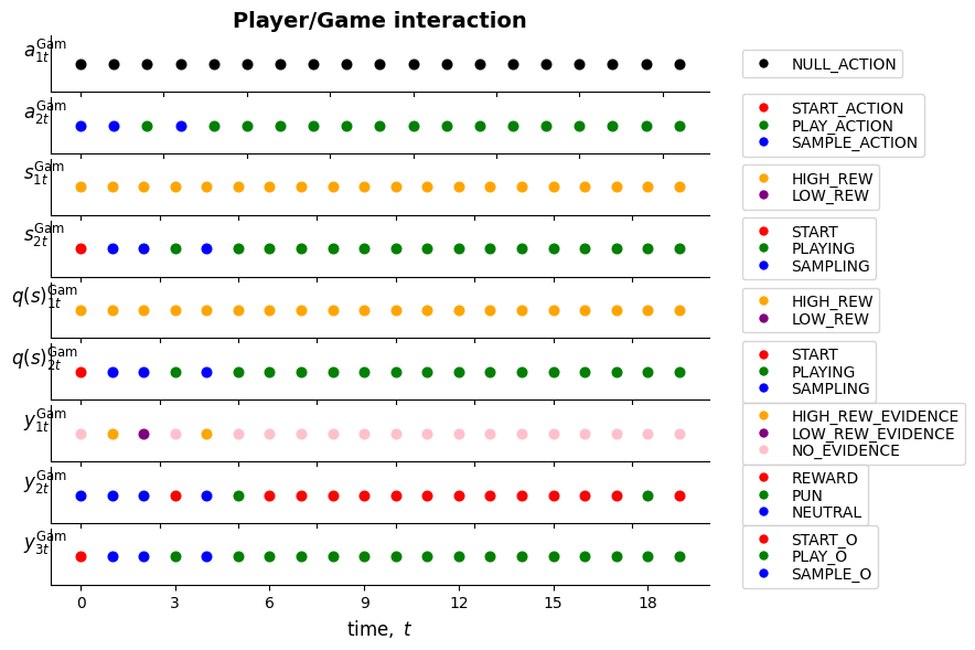
Beliefs: [('sᴳᵃᵐ₁', array([1., 0.])), ('sᴳᵃᵐ₂', array([0., 1., 0.]))]colors = [
{'NULL_ACTION':'black'},
{'START_ACTION':'red', 'PLAY_ACTION':'green', 'SAMPLE_ACTION': 'blue'},
{'HIGH_REW':'orange', 'LOW_REW':'purple'},
{'START':'red', 'PLAYING':'green', 'SAMPLING': 'blue'},
{'HIGH_REW':'orange', 'LOW_REW':'purple'},
{'START':'red', 'PLAYING':'green', 'SAMPLING': 'blue'},
{'HIGH_REW_EVIDENCE':'orange', 'LOW_REW_EVIDENCE':'purple', 'NO_EVIDENCE':'pink'},
{'REWARD':'red', 'PUN':'green', 'NEUTRAL': 'blue'},
{'START_O':'red', 'PLAY_O':'green', 'SAMPLE_O': 'blue'}
]
ylabel_size = 12
msi = 7 ## markersize for Line2D, diameter in points
siz = (msi/2)**2 * np.pi ## size for scatter, area of marker in points squared
fig = plt.figure(figsize=(9, 6))
## gs = GridSpec(6, 1, figure=fig, height_ratios=[1, 3, 1, 3, 3, 1])
gs = GridSpec(9, 1, figure=fig, height_ratios=[1, 1, 1, 1, 1, 1, 1, 1, 1])
ax = [fig.add_subplot(gs[i]) for i in range(9)]
i = 0
ax[i].set_title(f'Player/Game interaction', fontweight='bold',fontsize=14)
y_pos = 0
for t, s in zip(range(_T), _a_facs['aᴳᵃᵐ₁']): ## 'NULL'
ax[i].scatter(t, y_pos, color=colors[i][s], s=siz)
ax[i].set_ylabel('$a^{\mathrm{Gam}}_{1t}$', rotation=0, fontweight='bold', fontsize=ylabel_size)
ax[i].set_yticks([])
ax[i].set_xticklabels([])
leg_items = [
Line2D([0],[0],marker='o',color='w',markerfacecolor='black',markersize=msi,label='NULL_ACTION')]
ax[i].legend(handles=leg_items, bbox_to_anchor=(1.05, 0.5), loc='center left', borderaxespad=0, labelspacing=0.1)
ax[i].spines['top'].set_visible(False); ax[i].spines['right'].set_visible(False)
i = 1
y_pos = 0
for t, s in zip(range(_T), _a_facs['aᴳᵃᵐ₂']): ## 'PLAYING_VS_SAMPLING_CONTROL'
ax[i].scatter(t, y_pos, color=colors[i][s], s=siz, label=s)
ax[i].set_ylabel('$a^{\mathrm{Gam}}_{2t}$', rotation=0, fontweight='bold', fontsize=ylabel_size)
ax[i].set_yticks([])
leg_items = [
Line2D([0],[0],marker='o',color='w',markerfacecolor=colors[i]['START_ACTION'],markersize=msi,label='START_ACTION'),
Line2D([0],[0],marker='o',color='w',markerfacecolor=colors[i]['PLAY_ACTION'],markersize=msi,label='PLAY_ACTION'),
Line2D([0],[0],marker='o',color='w',markerfacecolor=colors[i]['SAMPLE_ACTION'],markersize=msi,label='SAMPLE_ACTION')]
ax[i].legend(handles=leg_items, bbox_to_anchor=(1.05, 0.5), loc='center left', borderaxespad=0, labelspacing=0.1)
ax[i].spines['top'].set_visible(False); ax[i].spines['right'].set_visible(False)
i = 2
y_pos = 0
for t, s in zip(range(_T), _s_facs['sᴳᵃᵐ₁']): ## 'GAME_STATE'
ax[i].scatter(t, y_pos, color=colors[i][s], s=siz)
ax[i].set_ylabel('$s^{\mathrm{Gam}}_{1t}$', rotation=0, fontweight='bold', fontsize=ylabel_size)
ax[i].set_yticks([])
ax[i].set_xticklabels([])
leg_items = [
Line2D([0],[0],marker='o',color='w',markerfacecolor=colors[i]['HIGH_REW'],markersize=msi,label='HIGH_REW'),
Line2D([0],[0],marker='o',color='w',markerfacecolor=colors[i]['LOW_REW'],markersize=msi,label='LOW_REW')]
ax[i].legend(handles=leg_items, bbox_to_anchor=(1.05, 0.5), loc='center left', borderaxespad=0, labelspacing=0.1)
ax[i].spines['top'].set_visible(False); ax[i].spines['right'].set_visible(False)
i = 3
y_pos = 0
for t, s in zip(range(_T), _s_facs['sᴳᵃᵐ₂']): ## 'PLAYING_VS_SAMPLING'
ax[i].scatter(t, y_pos, color=colors[i][s], s=siz, label=s)
ax[i].set_ylabel('$s^{\mathrm{Gam}}_{2t}$', rotation=0, fontweight='bold', fontsize=ylabel_size)
ax[i].set_yticks([])
leg_items = [
Line2D([0],[0],marker='o',color='w',markerfacecolor=colors[i]['START'],markersize=msi,label='START'),
Line2D([0],[0],marker='o',color='w',markerfacecolor=colors[i]['PLAYING'],markersize=msi,label='PLAYING'),
Line2D([0],[0],marker='o',color='w',markerfacecolor=colors[i]['SAMPLING'],markersize=msi,label='SAMPLING')]
ax[i].legend(handles=leg_items, bbox_to_anchor=(1.05, 0.5), loc='center left', borderaxespad=0, labelspacing=0.1)
ax[i].spines['top'].set_visible(False); ax[i].spines['right'].set_visible(False)
i = 4
y_pos = 0
for t, s in zip(range(_T), _s_facs['sᴳᵃᵐ₁']): ## 'GAME_STATE'
ax[i].scatter(t, y_pos, color=colors[i][s], s=siz)
ax[i].set_ylabel('$q(s)^{\mathrm{Gam}}_{1t}$', rotation=0, fontweight='bold', fontsize=ylabel_size)
ax[i].set_yticks([])
ax[i].set_xticklabels([])
leg_items = [
Line2D([0],[0],marker='o',color='w',markerfacecolor=colors[i]['HIGH_REW'],markersize=msi,label='HIGH_REW'),
Line2D([0],[0],marker='o',color='w',markerfacecolor=colors[i]['LOW_REW'],markersize=msi,label='LOW_REW')]
ax[i].legend(handles=leg_items, bbox_to_anchor=(1.05, 0.5), loc='center left', borderaxespad=0, labelspacing=0.1)
ax[i].spines['top'].set_visible(False); ax[i].spines['right'].set_visible(False)
i = 5
y_pos = 0
for t, s in zip(range(_T), _s_facs['sᴳᵃᵐ₂']): ## 'PLAYING_VS_SAMPLING'
ax[i].scatter(t, y_pos, color=colors[i][s], s=siz, label=s)
ax[i].set_ylabel('$q(s)^{\mathrm{Gam}}_{2t}$', rotation=0, fontweight='bold', fontsize=ylabel_size)
ax[i].set_yticks([])
leg_items = [
Line2D([0],[0],marker='o',color='w',markerfacecolor=colors[i]['START'],markersize=msi,label='START'),
Line2D([0],[0],marker='o',color='w',markerfacecolor=colors[i]['PLAYING'],markersize=msi,label='PLAYING'),
Line2D([0],[0],marker='o',color='w',markerfacecolor=colors[i]['SAMPLING'],markersize=msi,label='SAMPLING')]
ax[i].legend(handles=leg_items, bbox_to_anchor=(1.05, 0.5), loc='center left', borderaxespad=0, labelspacing=0.1)
ax[i].spines['top'].set_visible(False); ax[i].spines['right'].set_visible(False)
i = 6
y_pos = 0
for t, s in zip(range(_T), _y_mods['yᴳᵃᵐ₁']): ## 'GAME_STATE_OBS'
ax[i].scatter(t, y_pos, color=colors[i][s], s=siz, label=s)
ax[i].set_ylabel('$y^{\mathrm{Gam}}_{1t}$', rotation=0, fontweight='bold', fontsize=ylabel_size)
ax[i].set_yticks([])
leg_items = [
Line2D([0],[0],marker='o',color='w',markerfacecolor=colors[i]['HIGH_REW_EVIDENCE'],markersize=msi,label='HIGH_REW_EVIDENCE'),
Line2D([0],[0],marker='o',color='w',markerfacecolor=colors[i]['LOW_REW_EVIDENCE'],markersize=msi,label='LOW_REW_EVIDENCE'),
Line2D([0],[0],marker='o',color='w',markerfacecolor=colors[i]['NO_EVIDENCE'],markersize=msi,label='NO_EVIDENCE')]
ax[i].legend(handles=leg_items, bbox_to_anchor=(1.05, 0.5), loc='center left', borderaxespad=0, labelspacing=0.1)
ax[i].spines['top'].set_visible(False); ax[i].spines['right'].set_visible(False)
i = 7
y_pos = 0
for t, s in zip(range(_T), _y_mods['yᴳᵃᵐ₂']): ## 'GAME_OUTCOME'
ax[i].scatter(t, y_pos, color=colors[i][s], s=siz, label=s)
ax[i].set_ylabel('$y^{\mathrm{Gam}}_{2t}$', rotation=0, fontweight='bold', fontsize=ylabel_size)
ax[i].set_yticks([])
leg_items = [
Line2D([0],[0],marker='o',color='w',markerfacecolor=colors[i]['REWARD'],markersize=msi,label='REWARD'),
Line2D([0],[0],marker='o',color='w',markerfacecolor=colors[i]['PUN'],markersize=msi,label='PUN'),
Line2D([0],[0],marker='o',color='w',markerfacecolor=colors[i]['NEUTRAL'],markersize=msi,label='NEUTRAL')]
ax[i].legend(handles=leg_items, bbox_to_anchor=(1.05, 0.5), loc='center left', borderaxespad=0, labelspacing=0.1)
ax[i].spines['top'].set_visible(False); ax[i].spines['right'].set_visible(False)
i = 8
y_pos = 0
for t, s in zip(range(_T), _y_mods['yᴳᵃᵐ₃']): ## 'ACTION_SELF_OBS'
ax[i].scatter(t, y_pos, color=colors[i][s], s=siz, label=s)
ax[i].set_ylabel('$y^{\mathrm{Gam}}_{3t}$', rotation=0, fontweight='bold', fontsize=ylabel_size)
ax[i].set_yticks([])
leg_items = [
Line2D([0],[0],marker='o',color='w',markerfacecolor=colors[i]['START_O'],markersize=msi,label='START_O'),
Line2D([0],[0],marker='o',color='w',markerfacecolor=colors[i]['PLAY_O'],markersize=msi,label='PLAY_O'),
Line2D([0],[0],marker='o',color='w',markerfacecolor=colors[i]['SAMPLE_O'],markersize=msi,label='SAMPLE_O')]
ax[i].legend(handles=leg_items, bbox_to_anchor=(1.05, 0.5), loc='center left', borderaxespad=0, labelspacing=0.1)
ax[i].spines['top'].set_visible(False); ax[i].spines['right'].set_visible(False)
ax[i].xaxis.set_major_locator(MaxNLocator(integer=True))
## ax[i].xaxis.set_major_locator(MaxNLocator(nbins=10, integer=True))
ax[i].set_xlabel('$\mathrm{time,}\ t$', fontweight='bold', fontsize=12)
plt.tight_layout()
plt.subplots_adjust(hspace=0.1) ## Adjust this value as needed
plt.show()