Back to Blog | LearnableLoopAI.com | Portfolio of Projects |

In this post we use NumPyro to undertake a simple linear regression problem (based on McElreath’s book Statistical Rethinking). This Python library has a focus on stochastic variational inference (SVI). In the future it may be interesting to compare the performance of RxInfer with that of this more traditional approach.

Introduction to NumPyro for Probabilistic Programming and Bayesian Machine Learning

NumPyro is a cutting-edge probabilistic programming library that has gained significant traction in the field of Bayesian machine learning. Built on top of JAX, a high-performance numerical computing library, NumPyro offers a powerful and flexible framework for defining probabilistic models and performing efficient Bayesian inference. This introduction will explore NumPyro’s place in the broader context of probabilistic programming languages (PPLs) and Bayesian machine learning, highlighting its key features and advantages.

The Landscape of Probabilistic Programming Languages

Probabilistic programming languages have revolutionized the way researchers and practitioners approach Bayesian modeling and inference. These languages provide a high-level interface for specifying probabilistic models using familiar programming constructs, abstracting away much of the complexity involved in implementing inference algorithms.

Some notable PPLs in the ecosystem include:

Stan: A statically typed probabilistic programming language with its own domain-specific language (DSL).
PyMC: A Python library for probabilistic programming that offers a wide range of inference algorithms.
Pyro: A deep probabilistic programming library built on PyTorch, focusing on variational inference and deep generative models.
TensorFlow Probability: A library for probabilistic reasoning and statistical analysis in TensorFlow.

NumPyro enters this landscape as a modern, high-performance alternative that leverages the power of JAX for automatic differentiation and just-in-time (JIT) compilation.

NumPyro’s Distinctive Features

NumPyro distinguishes itself from other PPLs through several key features:

JAX Integration: By building on JAX, NumPyro inherits its ability to perform automatic differentiation, just-in-time compilation, and GPU/TPU acceleration. This integration allows for significant performance improvements, especially for large-scale models and datasets.
Familiar Syntax: NumPyro uses a Python-native syntax that will be familiar to users of other scientific computing libraries like NumPy. This ease of use lowers the barrier to entry for those new to probabilistic programming.
Flexible Model Specification: Users can define complex probabilistic models using a combination of NumPyro’s primitives and standard Python control flow.
Diverse Inference Algorithms: NumPyro supports a wide range of inference algorithms, including Markov Chain Monte Carlo (MCMC) methods like No U-Turn Sampler (NUTS) and Hamiltonian Monte Carlo (HMC), as well as variational inference techniques.
Automatic Guide Generation: For variational inference, NumPyro can automatically generate guide functions, simplifying the process of approximate inference for complex models.

NumPyro in Bayesian Machine Learning

In the context of Bayesian machine learning, NumPyro offers several advantages that make it an attractive choice for researchers and practitioners:

Scalability: The performance benefits from JAX allow NumPyro to scale efficiently to large datasets and complex models, making it suitable for modern machine learning tasks.
Flexibility in Model Design: NumPyro’s expressive model specification allows for the implementation of a wide range of Bayesian models, from simple linear regressions to complex hierarchical and time series models.
Integration with Machine Learning Workflows: Being a Python library, NumPyro integrates seamlessly with other popular machine learning and data science tools in the Python ecosystem.
Support for Bayesian Deep Learning: NumPyro can be used to implement Bayesian neural networks and other deep probabilistic models, leveraging JAX’s automatic differentiation capabilities.
Uncertainty Quantification: By providing full posterior distributions, NumPyro enables robust uncertainty quantification, which is crucial in many machine learning applications.

Applications and Use Cases

NumPyro’s capabilities make it suitable for a wide range of applications in Bayesian machine learning, including:

Hierarchical Modeling: For analyzing nested data structures common in fields like psychology, ecology, and social sciences.
Time Series Analysis: Implementing state-space models, dynamic linear models, and other time-dependent probabilistic models.
Bayesian Optimization: For hyperparameter tuning and experimental design optimization.
Causal Inference: Implementing causal models and performing counterfactual reasoning.
Bayesian Deep Learning: Creating uncertainty-aware neural networks and deep generative models.

Challenges and Considerations

While NumPyro offers many advantages, potential users should be aware of some challenges:

Learning Curve: Despite its familiar syntax, users new to probabilistic programming may face a learning curve in understanding Bayesian concepts and model specification.
JAX Dependency: While JAX provides performance benefits, it also introduces some constraints and may require users to adapt to its functional programming style.
Community and Ecosystem: Although growing, NumPyro’s ecosystem and community are still smaller compared to more established PPLs like Stan or PyMC.

Conclusion

NumPyro represents a significant advancement in the field of probabilistic programming and Bayesian machine learning. Its combination of a user-friendly interface, high performance, and flexibility makes it a powerful tool for a wide range of Bayesian modeling tasks. As the library continues to evolve and its community grows, NumPyro is poised to play an increasingly important role in the future of Bayesian machine learning and probabilistic programming.

import os
import warnings
import arviz as az
import matplotlib.pyplot as plt
import pandas as pd
import jax.numpy as jnp
from jax import random, vmap
import numpyro
import numpyro.distributions as dist
import numpyro.optim as optim
from numpyro.diagnostics import hpdi, print_summary
from numpyro.infer import Predictive, SVI, Trace_ELBO, init_to_value
from numpyro.infer.autoguide import AutoLaplaceApproximation
if "SVG" in os.environ:
    %config InlineBackend.figure_formats = ["svg"]
warnings.formatwarning = lambda message, category, *args, **kwargs: "{}: {}\n".format(
    category.__name__, message
)
az.style.use("arviz-darkgrid")
numpyro.set_platform("cpu")

A Gaussian model of height

The data

The dataset we use captures the height, weight, age, and gender census data of the Dobe Kung San tribe. This was compiled by Nancy Howell in the 1960s.

_df = pd.read_csv("workspace/kung-san.csv", sep=";")
_df

	height	weight	age	male
0	151.765	47.825606	63.0	1
1	139.700	36.485807	63.0	0
2	136.525	31.864838	65.0	0
3	156.845	53.041914	41.0	1
4	145.415	41.276872	51.0	0
...	...	...	...	...
539	145.415	31.127751	17.0	1
540	162.560	52.163080	31.0	1
541	156.210	54.062497	21.0	0
542	71.120	8.051258	0.0	1
543	158.750	52.531624	68.0	1

544 rows × 4 columns

_df.info()

<class 'pandas.core.frame.DataFrame'>
RangeIndex: 544 entries, 0 to 543
Data columns (total 4 columns):
 #   Column  Non-Null Count  Dtype  
---  ------  --------------  -----  
 0   height  544 non-null    float64
 1   weight  544 non-null    float64
 2   age     544 non-null    float64
 3   male    544 non-null    int64  
dtypes: float64(3), int64(1)
memory usage: 17.1 KB

print_summary(dict(zip(_df.columns, _df.T.values)), 0.89, False)


                mean       std    median      5.5%     94.5%     n_eff     r_hat
       age     29.34     20.75     27.00      0.00     57.00    186.38      1.03
    height    138.26     27.60    148.59     90.81    170.18    218.68      1.06
      male      0.47      0.50      0.00      0.00      1.00    670.75      1.00
    weight     35.61     14.72     40.06     11.37     55.71    305.62      1.05

Next, we sub-select the data to only contain datapoints where the age is greater or equal than 18:

_df2 = _df[_df.age >= 18]
_df2

	height	weight	age	male
0	151.765	47.825606	63.0	1
1	139.700	36.485807	63.0	0
2	136.525	31.864838	65.0	0
3	156.845	53.041914	41.0	1
4	145.415	41.276872	51.0	0
...	...	...	...	...
534	162.560	47.031821	27.0	0
537	142.875	34.246196	31.0	0
540	162.560	52.163080	31.0	1
541	156.210	54.062497	21.0	0
543	158.750	52.531624	68.0	1

352 rows × 4 columns

The model

We need some priors. The parameters to be estimated are \(\mu\) and \(\sigma\). Assuming these parameters are independent, we have

\[\begin{aligned} h_i &\sim \mathcal{N}(\mu, \sigma)\\ \mu &= \mathcal{N}(178, 20)\\ \sigma &\sim \mathcal{U}(0, 50) \end{aligned}\]

It is a good practice to plot the priors to get a sense of the assumptions they bring to the model.

_mu = jnp.linspace(100, 250, 101)
plt.plot(_mu, jnp.exp(dist.Normal(178, 20).log_prob(_mu)))
plt.show()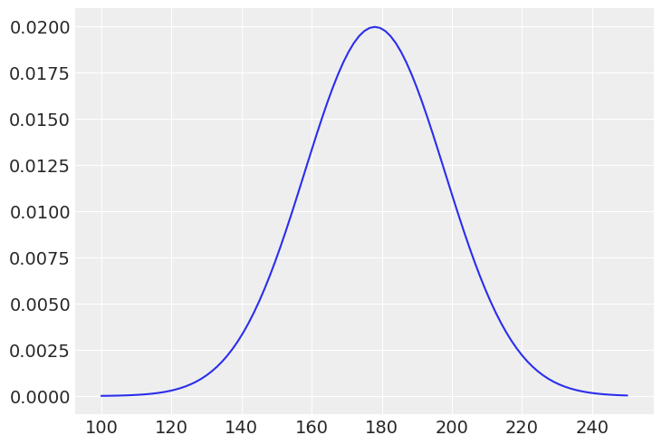

_sigma = jnp.linspace(-10, 60, 101)
plt.plot(_sigma, jnp.exp(dist.Uniform(0, 50, validate_args=True).log_prob(_sigma)))
plt.show()

UserWarning: Out-of-support values provided to log prob method. The value argument should be within the support.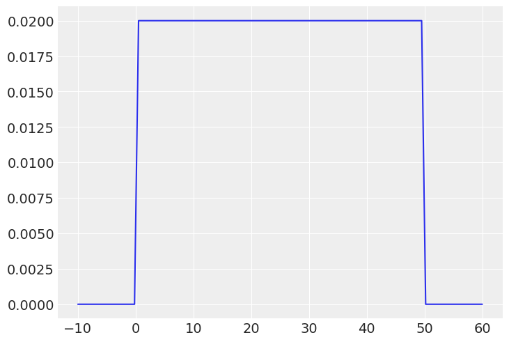

Next we will perform a prior predictive simulation to see what the priors imply about the distribution of heights.

_sample_mu = dist.Normal(178, 20).sample(random.PRNGKey(0), (int(1e4),))
_sample_sigma = dist.Uniform(0, 50).sample(random.PRNGKey(1), (int(1e4),))
_prior_h = dist.Normal(_sample_mu, _sample_sigma).sample(random.PRNGKey(2))
_ax = az.plot_kde(_prior_h)
_ax.set_xlabel('$\mathrm{height}, h$')
_ax.set_ylabel('$\mathrm{density}, p(h)$')
_ax.set_title(
    "$h ∼ \mathcal{N}(\mu, \sigma)$" + 
    "\n $μ ∼ \mathcal{N}(178, 20)$" +
    "\n $σ ∼ \mathcal{U}(0, 50)$"
)
plt.show()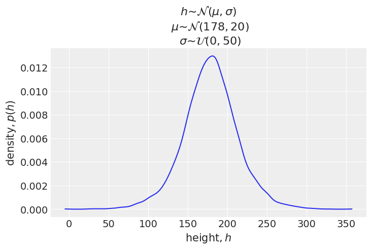

Consider the situation if we chose a different prior for \(\mu\) such that it has a much higher variance: \(\mu \sim \mathcal{N}(178, 100)\). Let’s do a prior predictive simulation again and look at the distribution of \(h\).

_sample_mu = dist.Normal(178, 100).sample(random.PRNGKey(0), (int(1e4),))
_prior_h = dist.Normal(_sample_mu, _sample_sigma).sample(random.PRNGKey(2))
_ax = az.plot_kde(_prior_h)
_ax.axvline(0, color='black', linestyle='--', lw=.5)
_ax.axvline(272, color='black', linestyle='-', lw=.5) ## Robert Wadlow height
_ax.set_xlabel('$\mathrm{height}, h$')
_ax.set_ylabel('$\mathrm{density}, p(h)$')
_ax.set_title(
    "$h ∼ \mathcal{N}(\mu, \sigma)$" + 
    "\n $μ ∼ \mathcal{N}(178, 100)$" +
    "\n $σ ∼ \mathcal{U}(0, 50)$"
)
plt.show()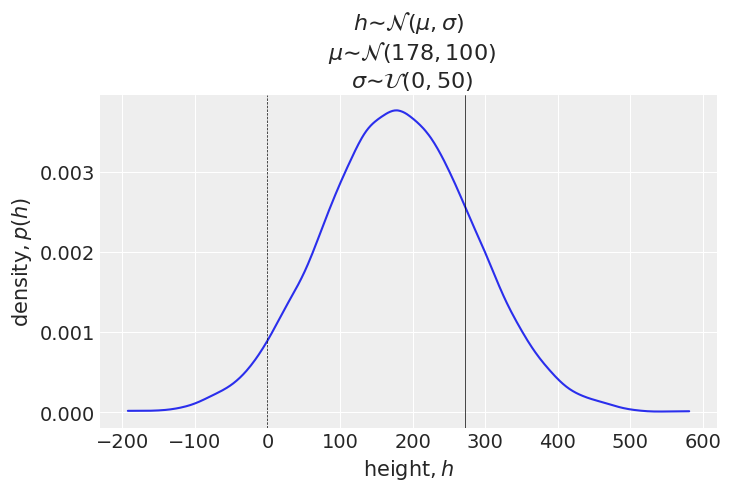

This time the height can have negative values (below dottd line). The solid line indicates the height of one of the tallest people in history - that of Robert Wadlow. His height was 272 cm. The simulation shows the many heights can exceed this height. Because we have a lot of data, using this rather silly prior won’t cause harm. However, there are situations where the choice of priors can have a significant effect.

Finding the posterior distribution with Laplace Approximation

From now on, we will use NumPyro’s formal mechanisms to provide an estimate of the posteriors we need. First we need to define a generative model inside a function that we call model(). Then we pass this function to the AutoLaplaceApproximation() function to create a guide. A guide is NumPyro’s name for a variational posterior. This created guide and well as the model is then passed on to the SVI’s constructor to provide an svi instance. Finally, we fit the model to the data.

Let’s implement the following generative model:

\[\begin{aligned} h_i &\sim \mathcal{N}(\mu, \sigma)\\ \mu &\sim \mathcal{N}(178, 20)\\ \sigma &\sim \mathcal{U}(0, 50) \end{aligned}\]

def model(height):
    mu = numpyro.sample("mu", dist.Normal(178, 20))
    sigma = numpyro.sample("sigma", dist.Uniform(0, 50))
    numpyro.sample("height", dist.Normal(mu, sigma), obs=height)

_guide = AutoLaplaceApproximation(model) ##. guide
_svi = SVI(
    model, ##. model
    _guide, ##. guide 
    optim.Adam(1), ##. optimizer 
    loss=Trace_ELBO(), 
    height=_df2.height.values)
_svi_result = _svi.run(random.PRNGKey(0), 2000)
_params = _svi_result.params

100%|██████████| 2000/2000 [00:00<00:00, 2453.58it/s, init loss: 4000.1155, avg. loss [1901-2000]: 1226.0389]

Now we look at the posterior distribution:

_post = _guide.sample_posterior(
    random.PRNGKey(1), 
    _params, ##. svi_result.params
    sample_shape=(1000,)
)
print_summary(_post, 0.89, False)


                mean       std    median      5.5%     94.5%     n_eff     r_hat
        mu    154.60      0.40    154.60    154.00    155.28    995.05      1.00
     sigma      7.76      0.30      7.76      7.33      8.26   1007.15      1.00

Next, we will change the prior for \(\mu\) to \(\mu \sim \mathcal{N}(178, 0.1)\).

def model(height):
    mu = numpyro.sample("mu", dist.Normal(178, 0.1)) ##. from 20 to 0.1
    sigma = numpyro.sample("sigma", dist.Uniform(0, 50))
    numpyro.sample("height", dist.Normal(mu, sigma), obs=height)

_guide = AutoLaplaceApproximation(model)
_svi = SVI(
    model, ##. model
    _guide, ##. guide
    optim.Adam(1), ##. optimizer
    loss=Trace_ELBO(), 
    height=_df2.height.values
)
_svi_result = _svi.run(random.PRNGKey(0), 2000)
_params = _svi_result.params

100%|██████████| 2000/2000 [00:00<00:00, 2788.43it/s, init loss: 1584193.6250, avg. loss [1901-2000]: 1626.5830]

_post = _guide.sample_posterior(
    random.PRNGKey(1), 
    _params, ##. svi_result.params
    sample_shape=(1000,)
)
print_summary(_post, 0.89, False)


                mean       std    median      5.5%     94.5%     n_eff     r_hat
        mu    177.86      0.10    177.86    177.72    178.03    995.05      1.00
     sigma     24.57      0.94     24.60     23.01     25.96   1012.88      1.00

Linear prediction

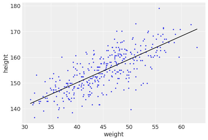
So far, we have only built a probabilistic model of the height of the adult population. Next we will look at how weight is related to height by means of a linear regression.

az.plot_pair(_df2[["weight", "height"]].to_dict(orient="list"))
plt.show()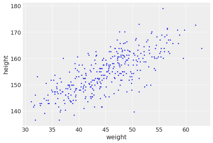

The linear model strategy

Our strategy is to make the mean parameter \(\mu\) into a linear function of the predictor variable (weight), and some other parameters that we will invent. Using \(x\) for the weight, and \(\bar x\) for its average, we come up with the following probabilistic model:

\[\begin{align} h_i &\sim \mathcal{N}(\mu_i, \sigma) \tag{likelihood} \\ \mu_i &= \alpha + \beta(x_i - \bar{x}) \tag{linear model} \\ \alpha &\sim \mathcal{N}(178, 20) \tag{prior} \\ \beta &\sim \mathcal{N}(0, 10) \tag{prior} \\ \sigma &\sim \mathcal{U}(0, 50) \tag{prior} \end{align}\]

Let’s simulate the lines implied by the priors for \(\alpha\) and \(\beta\):

with numpyro.handlers.seed(rng_seed=2971):
    _N = 100 ## 100 lines
    _a = numpyro.sample("a", dist.Normal(178, 20).expand([_N]))
    _b = numpyro.sample("b", dist.Normal(0, 10).expand([_N]))

plt.subplot(
    xlim=(_df2.weight.min(), _df2.weight.max()),
    ylim=(-100, 400),
    xlabel="weight",
    ylabel="height",
)
plt.axhline(y=0, c="k", ls="--")
plt.axhline(y=272, c="k", ls="-", lw=0.5)
plt.title("$b \sim \mathcal{N}(0, 10)$") ##.
_xbar = _df2.weight.mean()
_x = jnp.linspace(_df2.weight.min(), _df2.weight.max(), 101)
for i in range(_N):
    plt.plot(_x, _a[i] + _b[i]*(_x - _xbar), "k", alpha=0.2)
plt.show()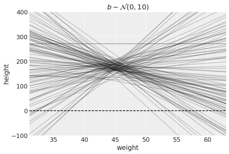

Average height increases with average weight, so let’s restrict it to positive values by using a log-normal prior for \(\beta\):

\[\beta \sim \mathcal{L}\mathcal{N}(0, 1)\]

_b = dist.LogNormal(0, 1).sample(random.PRNGKey(0), (int(1e4),))
az.plot_kde(_b)
plt.show()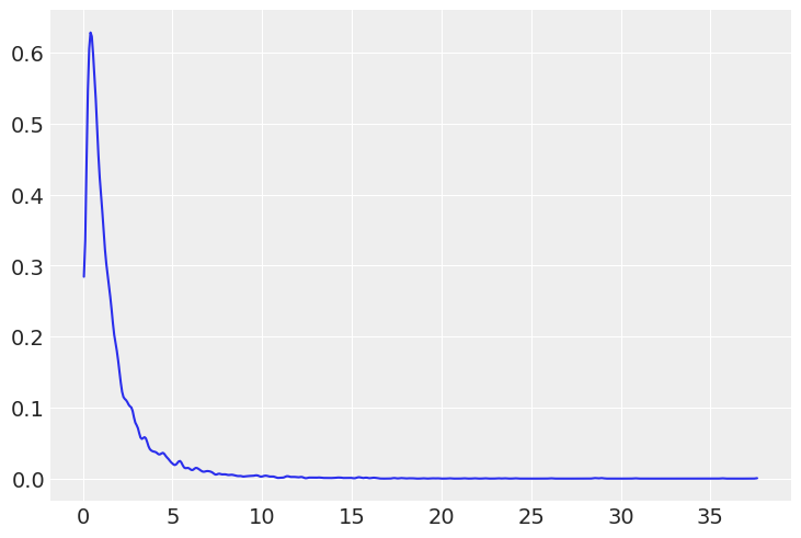

We do the prior predictive simulation again, using the log-normal prior:

with numpyro.handlers.seed(rng_seed=2971):
    _N = 100 ## 100 lines
    _a = numpyro.sample("a", dist.Normal(178, 28).expand([_N]))
    _b = numpyro.sample("b", dist.LogNormal(0, 1).expand([_N]))

plt.subplot(
    xlim=(_df2.weight.min(), _df2.weight.max()),
    ylim=(-100, 400),
    xlabel="weight",
    ylabel="height",
)
plt.axhline(y=0, c="k", ls="--")
plt.axhline(y=272, c="k", ls="-", lw=0.5)
plt.title("$\mathrm{log}(b) \sim \mathcal{N}(0, 1)$") ##.
_xbar = _df2.weight.mean()
_x = jnp.linspace(_df2.weight.min(), _df2.weight.max(), 101)
for i in range(_N):
    plt.plot(_x, _a[i] + _b[i]*(_x - _xbar), "k", alpha=0.2)
plt.show()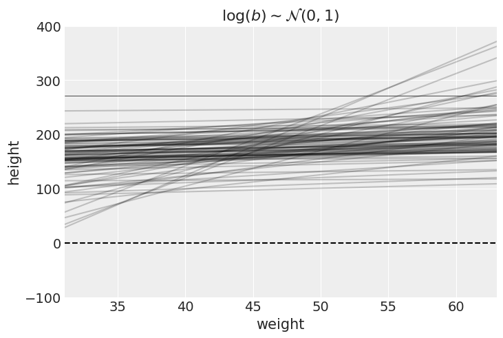

Finding the posterior distribution

Using the latest model, we find the posterior distribution again:

\[\begin{aligned} h_i &\sim \mathcal{N}(\mu_i, \sigma)\\ \mu_i &= \alpha + \beta(x_i - \bar{x})\\ \alpha &\sim \mathcal{N}(178, 20)\\ \beta &\sim \mathcal{LN}(0, 1)\\ \sigma &\sim \mathcal{U}(0, 50) \end{aligned}\]

## fit model
def model(weight, height):
    a = numpyro.sample("a", dist.Normal(178, 20))
    b = numpyro.sample("b", dist.LogNormal(0, 1))
    sigma = numpyro.sample("sigma", dist.Uniform(0, 50))
    mu = numpyro.deterministic("mu", a + b*(weight - _xbar))
    numpyro.sample("height", dist.Normal(mu, sigma), obs=height)

_guide = AutoLaplaceApproximation(model)
_svi = SVI(
    model, ##. model
    _guide, ##. guide
    optim.Adam(1),
    loss=Trace_ELBO(),
    weight=_df2.weight.values,
    height=_df2.height.values,
)
_svi_result = _svi.run(random.PRNGKey(0), 2000)
_params = _svi_result.params

100%|██████████| 2000/2000 [00:00<00:00, 2056.22it/s, init loss: 40631.5391, avg. loss [1901-2000]: 1078.9297]

_samples = _guide.sample_posterior(
    random.PRNGKey(1), 
    _params, 
    sample_shape=(1000,)
)
_samples.pop("mu")
print_summary(_samples, 0.89, False)


                mean       std    median      5.5%     94.5%     n_eff     r_hat
         a    154.62      0.27    154.63    154.16    155.03    931.50      1.00
         b      0.91      0.04      0.90      0.84      0.97   1083.74      1.00
     sigma      5.08      0.19      5.08      4.79      5.41    949.65      1.00

Finally, we plot the posterior inference against the data:

az.plot_pair(_df2[["weight", "height"]].to_dict(orient="list"))
_post = _guide.sample_posterior(
    random.PRNGKey(1), 
    _params, 
    sample_shape=(1000,)
)
_a_map = jnp.mean(_post["a"])
_b_map = jnp.mean(_post["b"])
_x = jnp.linspace(_df2.weight.min(), _df2.weight.max(), 101)
plt.plot(_x, _a_map + _b_map*(_x - _xbar), "k")
plt.show()